Now You Flipped Your 2 Coins Again but You Did It 100 Times

The Chi-Square Distribution

Goodness-of-Fit Test

In this type of hypothesis test, you lot determine whether the data "fit" a particular distribution or not. For instance, you may suspect your unknown information fit a binomial distribution. You lot utilise a chi-foursquare test (significant the distribution for the hypothesis examination is chi-foursquare) to decide if there is a fit or not. The null and the alternative hypotheses for this exam may exist written in sentences or may be stated every bit equations or inequalities.

The exam statistic for a goodness-of-fit test is:

where:

• O = observed values (data)
• E = expected values (from theory)
• yard = the number of different data cells or categories

The observed values are the information values and the expected values are the values yous would expect to become if the null hypothesis were truthful. There are north terms of the course .

The number of degrees of freedom is df = (number of categories – 1).

The goodness-of-fit test is almost always right-tailed. If the observed values and the corresponding expected values are not close to each other, then the exam statistic can get very big and will exist way out in the right tail of the chi-square curve.

Note

The expected value for each cell needs to be at least five in order for you to use this test.

Absence of college students from math classes is a major concern to math instructors because missing class appears to increment the drop rate. Suppose that a study was done to determine if the actual student absence rate follows faculty perception. The faculty expected that a group of 100 students would miss form co-ordinate to (Effigy).

Number of absences per term	Expected number of students
0–2	fifty
three–5	30
half dozen–eight	12
9–11	half dozen
12+	two

A random survey across all mathematics courses was and then done to determine the bodily number (observed) of absences in a course. The chart in (Figure) displays the results of that survey.

Number of absences per term	Actual number of students
0–2	35
3–v	40
half dozen–8	20
9–11	1
12+	4

Make up one's mind the null and culling hypotheses needed to bear a goodness-of-fit exam.

H₀ : Educatee absenteeism fits kinesthesia perception.

The alternative hypothesis is the opposite of the zip hypothesis.

H_a : Student absenteeism does not fit kinesthesia perception.

a. Tin can you apply the information as it appears in the charts to conduct the goodness-of-fit test?

a. No. Notice that the expected number of absences for the "12+" entry is less than five (it is ii). Combine that grouping with the "9–11" group to create new tables where the number of students for each entry are at to the lowest degree five. The new results are in (Figure) and (Figure).

Number of absences per term	Expected number of students
0–2	50
3–5	30
6–8	12
9+	8

Number of absences per term	Actual number of students
0–ii	35
3–5	xl
6–viii	20
9+	5

b. What is the number of degrees of freedom (df)?

b. There are four "cells" or categories in each of the new tables.

df = number of cells – 1 = iv – i = 3

Endeavour Information technology

A factory managing director needs to empathise how many products are lacking versus how many are produced. The number of expected defects is listed in (Figure).

Number produced	Number defective
0–100	5
101–200	half-dozen
201–300	7
301–400	8
401–500	10

A random sample was taken to make up one's mind the bodily number of defects. (Figure) shows the results of the survey.

Number produced	Number defective
0–100	5
101–200	7
201–300	8
301–400	ix
401–500	11

Country the null and alternative hypotheses needed to bear a goodness-of-fit test, and state the degrees of freedom.

Employers want to know which days of the calendar week employees are absent in a five-day work week. Near employers would like to believe that employees are absent-minded equally during the week. Suppose a random sample of lx managers were asked on which day of the week they had the highest number of employee absences. The results were distributed as in (Effigy). For the population of employees, do the days for the highest number of absences occur with equal frequencies during a 5-day work week? Test at a 5% significance level.

Day of the Week Employees were Well-nigh Absent-minded

	Monday	Tuesday	Wednesday	Thursday	Friday
Number of Absences	xv	12	9	nine	15

The nada and culling hypotheses are:

• H₀ : The absent days occur with equal frequencies, that is, they fit a uniform distribution.
• H_a : The absent days occur with diff frequencies, that is, they do not fit a uniform distribution.

If the absent days occur with equal frequencies, then, out of threescore absent days (the total in the sample: fifteen + 12 + 9 + 9 + 15 = sixty), there would be 12 absences on Monday, 12 on Tuesday, 12 on Wednesday, 12 on Thursday, and 12 on Friday. These numbers are the expected (E) values. The values in the tabular array are the observed (O) values or information.

This time, calculate the χ ² test statistic by hand. Make a chart with the post-obit headings and fill in the columns:

• Expected (E) values (12, 12, 12, 12, 12)
• Observed (O) values (15, 12, 9, 9, 15)
• (O – Eastward)
• (O – E)²
• 

Now add (sum) the last column. The sum is three. This is the χⁱⁱ examination statistic.

To find the p-value, calculate P(χ ² > three). This examination is right-tailed. (Employ a computer or computer to find the p-value. You should get p-value = 0.5578.)

The dfs are the number of cells – i = 5 – 1 = iv

Press 2nd DISTR. Arrow downwards to χiicdf. Press ENTER. Enter (3,x^99,4). Rounded to four decimal places, you should see 0.5578, which is the p-value.

Next, complete a graph like the post-obit one with the proper labeling and shading. (Y'all should shade the right tail.)

The decision is non to decline the null hypothesis.

Decision: At a 5% level of significance, from the sample data, at that place is non sufficient evidence to conclude that the absent days exercise not occur with equal frequencies.

TI-83+ and some TI-84 calculators practice not accept a special program for the examination statistic for the goodness-of-fit test. The next example (Figure) has the calculator instructions. The newer TI-84 calculators have in STAT TESTS the test Chi2 GOF. To run the test, put the observed values (the data) into a first listing and the expected values (the values you expect if the null hypothesis is true) into a 2nd list. Press STAT TESTS and Chi2 GOF. Enter the list names for the Observed listing and the Expected list. Enter the degrees of freedom and printing summate or draw. Make sure yous articulate any lists before you commencement. To Clear Lists in the calculators: Go into STAT EDIT and arrow upwards to the list name area of the detail list. Press Clear and so arrow down. The list will be cleared. Alternatively, you can press STAT and press 4 (for ClrList). Enter the list name and printing ENTER.

Endeavour Information technology

Teachers want to know which night each week their students are doing most of their homework. Nearly teachers think that students do homework equally throughout the week. Suppose a random sample of 56 students were asked on which night of the week they did the about homework. The results were distributed as in (Figure).

	Sunday	Monday	Tuesday	Wednesday	Thursday	Fri	Sabbatum
Number of Students	11	8	ten	7	10	5	5

From the population of students, do the nights for the highest number of students doing the majority of their homework occur with equal frequencies during a calendar week? What type of hypothesis exam should you use?

One study indicates that the number of televisions that American families have is distributed (this is the given distribution for the American population) as in (Figure).

Number of Televisions	Percent
0	10
ane	16
2	55
three	11
four+	viii

The table contains expected (Due east) percents.

A random sample of 600 families in the far western Usa resulted in the information in (Effigy).

Number of Televisions	Frequency
	Total = 600
0	66
1	119
2	340
3	60
4+	xv

The table contains observed (O) frequency values.

At the one% significance level, does it announced that the distribution "number of televisions" of far western United States families is different from the distribution for the American population every bit a whole?

This trouble asks yous to examination whether the far western United states of america families distribution fits the distribution of the American families. This test is always right-tailed.

The first table contains expected percentages. To go expected (E) frequencies, multiply the percentage by 600. The expected frequencies are shown in (Figure).

Number of Televisions	Percent	Expected Frequency
0	10	(0.x)(600) = 60
1	xvi	(0.16)(600) = 96
2	55	(0.55)(600) = 330
3	xi	(0.11)(600) = 66
over iii	8	(0.08)(600) = 48

Therefore, the expected frequencies are 60, 96, 330, 66, and 48. In the TI calculators, you tin can allow the computer do the math. For example, instead of 60, enter 0.ten*600.

H₀ : The "number of televisions" distribution of far western United States families is the aforementioned as the "number of televisions" distribution of the American population.

H_a : The "number of televisions" distribution of far western Us families is different from the "number of televisions" distribution of the American population.

Distribution for the examination: where df = (the number of cells) – 1 = 5 – 1 = 4.

Calculate the exam statistic: χii = 29.65

Graph:

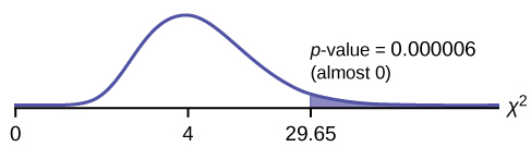
Probability statement: p-value = P(χ ² > 29.65) = 0.000006

Compare α and the p-value:

• α = 0.01
• p-value = 0.000006

So, α > p-value.

Make a decision: Since α > p-value, turn down H_o .

This ways you turn down the belief that the distribution for the far western states is the same every bit that of the American population as a whole.

Conclusion: At the i% significance level, from the data, there is sufficient evidence to conclude that the "number of televisions" distribution for the far western United States is dissimilar from the "number of televisions" distribution for the American population every bit a whole.

Printing STAT and ENTER. Make certain to clear lists L1, L2, and L3 if they have data in them (meet the note at the stop of (Figure)). Into L1, put the observed frequencies 66, 119, 349, 60, xv. Into L2, put the expected frequencies .10*600, .16*600, .55*600, .11*600, .08*600. Arrow over to list L3 and up to the name expanse "L3". Enter (L1-L2)^2/L2 and ENTER. Printing 2nd QUIT. Printing 2nd LIST and arrow over to MATH. Press 5. Yous should encounter "sum" (Enter L3). Rounded to 2 decimal places, you should see 29.65. Press second DISTR. Press 7 or Arrow down to 7:χ2cdf and press ENTER. Enter (29.65,1E99,4). Rounded to four places, you should see v.77E-vi = .000006 (rounded to six decimal places), which is the p-value.

The newer TI-84 calculators have in STAT TESTS the test Chi2 GOF. To run the test, put the observed values (the data) into a first list and the expected values (the values you lot expect if the zippo hypothesis is true) into a 2d list. Press STAT TESTS and Chi2 GOF. Enter the list names for the Observed listing and the Expected list. Enter the degrees of freedom and press calculate or depict. Make sure y'all articulate whatsoever lists before y'all get-go.

Try It

The expected percentage of the number of pets students have in their homes is distributed (this is the given distribution for the student population of the U.s.) as in (Figure).

Number of Pets	Percentage
0	18
one	25
two	30
3	eighteen
4+	nine

A random sample of 1,000 students from the Eastern Us resulted in the data in (Figure).

Number of Pets	Frequency
0	210
i	240
ii	320
3	140
iv+	90

At the 1% significance level, does information technology announced that the distribution "number of pets" of students in the Eastern United States is different from the distribution for the United states of america pupil population as a whole? What is the p-value?

Suppose you flip 2 coins 100 times. The results are 20 HH, 27 HT, 30 TH, and 23 TT. Are the coins fair? Test at a five% significance level.

This problem can be set as a goodness-of-fit problem. The sample infinite for flipping two off-white coins is {HH, HT, Thursday, TT}. Out of 100 flips, you would expect 25 HH, 25 HT, 25 TH, and 25 TT. This is the expected distribution. The question, "Are the coins fair?" is the same as saying, "Does the distribution of the coins (20 HH, 27 HT, 30 Thursday, 23 TT) fit the expected distribution?"

Random Variable: Let X = the number of heads in 1 flip of the 2 coins. 10 takes on the values 0, 1, two. (There are 0, 1, or 2 heads in the flip of ii coins.) Therefore, the number of cells is three. Since X = the number of heads, the observed frequencies are 20 (for two heads), 57 (for one head), and 23 (for zero heads or both tails). The expected frequencies are 25 (for two heads), 50 (for ane head), and 25 (for zero heads or both tails). This exam is correct-tailed.

H₀ : The coins are fair.

H_a : The coins are non fair.

Distribution for the test: where df = three – 1 = 2.

Calculate the test statistic: χ ^two = 2.14

Graph:

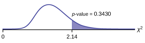
Probability statement: p-value = P(χ ^two > 2.14) = 0.3430

Compare α and the p-value:

• α = 0.05
• p-value = 0.3430

α < p-value.

Make a decision: Since α < p-value, do not reject H₀ .

Conclusion: There is insufficient show to conclude that the coins are not fair.

Press STAT and ENTER. Brand certain you clear lists L1, L2, and L3 if they have data in them. Into L1, put the observed frequencies 20, 57, 23. Into L2, put the expected frequencies 25, 50, 25. Arrow over to listing L3 and upwards to the name area "L3". Enter (L1-L2)^2/L2 and ENTER. Press second QUIT. Press second LIST and pointer over to MATH. Printing 5. You lot should see "sum".Enter L3. Rounded to two decimal places, y'all should see 2.14. Press 2nd DISTR. Arrow down to 7:χ2cdf (or press seven). Press ENTER. Enter two.xiv,1E99,2). Rounded to four places, you should see .3430, which is the p-value.

The newer TI-84 calculators take in STAT TESTS the examination Chi2 GOF. To run the exam, put the observed values (the data) into a offset list and the expected values (the values you look if the zip hypothesis is true) into a second list. Press STAT TESTS and Chi2 GOF. Enter the list names for the Observed list and the Expected listing. Enter the degrees of freedom and press calculate or draw. Make sure you clear any lists before y'all beginning.

Try It

Students in a social studies class hypothesize that the literacy rates across the earth for every region are 82%. (Figure) shows the actual literacy rates across the world broken down past region. What are the examination statistic and the degrees of freedom?

MDG Region	Developed Literacy Charge per unit (%)
Developed Regions	99.0
Commonwealth of Independent States	99.5
Northern Africa	67.iii
Sub-Saharan Africa	62.5
Latin America and the Caribbean area	91.0
Eastern asia	93.8
South asia	61.9
Due south-Eastern Asia	91.9
Western asia	84.five
Oceania	66.4

Chapter Review

To assess whether a data set fits a specific distribution, you can utilize the goodness-of-fit hypothesis examination that uses the chi-foursquare distribution. The zero hypothesis for this test states that the information come from the assumed distribution. The test compares observed values against the values you would expect to have if your information followed the causeless distribution. The test is almost e'er correct-tailed. Each ascertainment or cell category must have an expected value of at to the lowest degree 5.

Formula Review

goodness-of-fit test statistic where:

O: observed values
E: expected values

k: number of different data cells or categories

df = grand − 1 degrees of freedom

Determine the advisable examination to exist used in the next iii exercises.

An archeologist is computing the distribution of the frequency of the number of artifacts she finds in a dig site. Based on previous digs, the archaeologist creates an expected distribution broken downwardly by grid sections in the dig site. Once the site has been fully excavated, she compares the bodily number of artifacts found in each filigree section to see if her expectation was accurate.

An economist is deriving a model to predict outcomes on the stock market. He creates a list of expected points on the stock market alphabetize for the adjacent two weeks. At the close of each day'due south trading, he records the actual points on the index. He wants to encounter how well his model matched what actually happened.

a goodness-of-fit examination

A personal trainer is putting together a weight-lifting program for her clients. For a 90-day program, she expects each client to lift a specific maximum weight each week. Equally she goes along, she records the actual maximum weights her clients lifted. She wants to know how well her expectations met with what was observed.

Use the post-obit data to answer the next five exercises: A teacher predicts that the distribution of grades on the final examination volition be and they are recorded in (Figure).

Grade	Proportion
A	0.25
B	0.30
C	0.35
D	0.x

The actual distribution for a class of 20 is in (Figure).

Grade	Frequency
A	7
B	7
C	five
D	ane

______

3

State the nix and alternative hypotheses.

χ² test statistic = ______

2.04

At the 5% significance level, what can y'all conclude?

We turn down to reject the goose egg hypothesis. There is not plenty evidence to advise that the observed examination scores are significantly different from the expected examination scores.

Employ the post-obit data to respond the side by side nine exercises: The following data are real. The cumulative number of AIDS cases reported for Santa Clara County is broken downwardly past ethnicity equally in (Figure).

Ethnicity	Number of Cases
White	two,229
Hispanic	1,157
Black/African-American	457
Asian, Pacific Islander	232
	Total = 4,075

The per centum of each ethnic group in Santa Clara County is as in (Effigy).

Ethnicity	Per centum of total county population	Number expected (round to two decimal places)
White	42.nine%	1748.18
Hispanic	26.7%
Black/African-American	2.6%
Asian, Pacific Islander	27.8%
	Total = 100%

If the ethnicities of AIDS victims followed the ethnicities of the total county population, fill in the expected number of cases per ethnic grouping.
Perform a goodness-of-fit test to determine whether the occurrence of AIDS cases follows the ethnicities of the full general population of Santa Clara County.

H₀ : _______

H₀ : the distribution of AIDS cases follows the ethnicities of the general population of Santa Clara County.

Is this a right-tailed, left-tailed, or 2-tailed exam?

right-tailed

degrees of freedom = _______

χ^two exam statistic = _______

2016.136

Graph the state of affairs. Label and calibration the horizontal axis. Mark the mean and test statistic. Shade in the region respective to the p-value.

Let α = 0.05

Conclusion: ________________

Reason for the Determination: ________________

Conclusion (write out in complete sentences): ________________

Graph: Check student's solution.

Conclusion: Turn down the null hypothesis.

Reason for the Determination: p-value < alpha

Conclusion (write out in complete sentences): The make-upwards of AIDS cases does not fit the ethnicities of the full general population of Santa Clara County.

Does it appear that the pattern of AIDS cases in Santa Clara County corresponds to the distribution of ethnic groups in this county? Why or why non?

Homework

For each problem, use a solution canvas to solve the hypothesis test problem. Go to (Figure) for the chi-foursquare solution canvass. Round expected frequency to two decimal places.

A half dozen-sided dice is rolled 120 times. Fill in the expected frequency cavalcade. Then, deport a hypothesis exam to determine if the die is off-white. The data in (Figure) are the issue of the 120 rolls.

Face Value	Frequency	Expected Frequency
ane	xv
ii	29
3	16
4	fifteen
5	30
6	15

The marital condition distribution of the U.South. male population, ages fifteen and older, is as shown in (Figure).

Marital Status	Pct	Expected Frequency
never married	31.three
married	56.one
widowed	2.5
divorced/separated	10.1

Suppose that a random sample of 400 U.Southward. young adult males, 18 to 24 years old, yielded the following frequency distribution. Nosotros are interested in whether this age group of males fits the distribution of the U.Southward. developed population. Calculate the frequency one would expect when surveying 400 people. Fill in (Effigy), rounding to two decimal places.

Marital Status	Frequency
never married	140
married	238
widowed	2
divorced/separated	20

Marital Condition	Pct	Expected Frequency
never married	31.3	125.2
married	56.1	224.4
widowed	two.5	ten
divorced/separated	ten.1	twoscore.iv

1. The data fits the distribution.
2. The data does not fit the distribution.
3. 3
4. chi-square distribution with df = 3
5. xix.27
6. 0.0002
7. Check pupil's solution.
8. 1. Alpha = 0.05
   2. Decision: Decline nil
   3. Reason for determination: p-value < alpha
   4. Conclusion: Data does non fit the distribution.

Use the following data to respond the side by side two exercises: The columns in (Figure) contain the Race/Ethnicity of U.Due south. Public Schools for a recent year, the percentages for the Advanced Placement Examinee Population for that course, and the Overall Student Population. Suppose the right column contains the result of a survey of one,000 local students from that year who took an AP Exam.

Race/Ethnicity	AP Examinee Population	Overall Pupil Population	Survey Frequency
Asian, Asian American, or Pacific Islander	x.ii%	5.iv%	113
Black or African-American	8.2%	14.5%	94
Hispanic or Latino	fifteen.v%	15.9%	136
American Indian or Alaska Native	0.vi%	1.2%	x
White	59.4%	61.6%	604
Not reported/other	6.ane%	i.iv%	43

Perform a goodness-of-fit exam to determine whether the local results follow the distribution of the U.S. overall educatee population based on ethnicity.

Perform a goodness-of-fit exam to make up one's mind whether the local results follow the distribution of U.S. AP examinee population, based on ethnicity.

1. H₀ : The local results follow the distribution of the U.Southward. AP examinee population
2. H_a : The local results do non follow the distribution of the U.S. AP examinee population
3. df = 5
4. chi-foursquare distribution with df = 5
5. chi-foursquare exam statistic = xiii.4
6. p-value = 0.0199
7. Check pupil's solution.
8. 1. Alpha = 0.05
   2. Decision: Reject null when a = 0.05
   3. Reason for Decision: p-value < alpha
   4. Conclusion: Local data practise not fit the AP Examinee Distribution.
   5. Conclusion: Do not reject null when a = 0.01
   6. Conclusion: In that location is insufficient prove to conclude that local data do not follow the distribution of the U.S. AP examinee distribution.

The City of South Lake Tahoe, CA, has an Asian population of 1,419 people, out of a total population of 23,609. Suppose that a survey of ane,419 self-reported Asians in the Manhattan, NY, area yielded the data in (Figure). Conduct a goodness-of-fit exam to determine if the self-reported sub-groups of Asians in the Manhattan area fit that of the Lake Tahoe area.

Race	Lake Tahoe Frequency	Manhattan Frequency
Asian Indian	131	174
Chinese	118	557
Filipino	one,045	518
Japanese	80	54
Korean	12	29
Vietnamese	9	21
Other	24	66

Use the post-obit data to answer the side by side two exercises: UCLA conducted a survey of more than 263,000 college freshmen from 385 colleges in autumn 2005. The results of students' expected majors past gender were reported in The Chronicle of Higher Education (2/ii/2006) . Suppose a survey of 5,000 graduating females and 5,000 graduating males was done as a follow-upwardly last year to determine what their actual majors were. The results are shown in the tables for (Figure) and (Figure). The second column in each table does not add to 100% because of rounding.

Conduct a goodness-of-fit test to make up one's mind if the actual college majors of graduating females fit the distribution of their expected majors.

Major	Women – Expected Major	Women – Bodily Major
Arts & Humanities	fourteen.0%	670
Biological Sciences	viii.4%	410
Business	xiii.1%	685
Education	13.0%	650
Engineering	2.half-dozen%	145
Physical Sciences	2.6%	125
Professional	18.9%	975
Social Sciences	13.0%	605
Technical	0.4%	15
Other	5.8%	300
Undecided	8.0%	420

1. H₀ : The actual college majors of graduating females fit the distribution of their expected majors
2. H_a : The actual college majors of graduating females do non fit the distribution of their expected majors
3. df = ten
4. chi-square distribution with df = 10
5. test statistic = eleven.48
6. p-value = 0.3211
7. Check student's solution.
8. 1. Alpha = 0.05
   2. Conclusion: Do non reject null when a = 0.05 and a = 0.01
   3. Reason for decision: p-value > alpha
   4. Conclusion: There is insufficient bear witness to conclude that the distribution of bodily college majors of graduating females do non fit the distribution of their expected majors.

Conduct a goodness-of-fit test to determine if the bodily college majors of graduating males fit the distribution of their expected majors.

Major	Men – Expected Major	Men – Bodily Major
Arts & Humanities	11.0%	600
Biological Sciences	6.7%	330
Business	22.7%	1130
Education	5.8%	305
Engineering	15.6%	800
Physical Sciences	3.half dozen%	175
Professional	9.iii%	460
Social Sciences	7.6%	370
Technical	ane.8%	xc
Other	8.2%	400
Undecided	6.half-dozen%	340

Read the argument and decide whether it is true or false.

In a goodness-of-fit exam, the expected values are the values we would wait if the aught hypothesis were true.

true

In general, if the observed values and expected values of a goodness-of-fit exam are non shut together, then the exam statistic tin can get very large and on a graph will be way out in the right tail.

Use a goodness-of-fit test to make up one's mind if high school principals believe that students are absent as during the week or not.

true

The test to use to determine if a six-sided die is fair is a goodness-of-fit test.

In a goodness-of fit examination, if the p-value is 0.0113, in general, do not pass up the goose egg hypothesis.

fake

A sample of 212 commercial businesses was surveyed for recycling one commodity; a article hither ways any one type of recyclable material such as plastic or aluminum. (Figure) shows the business categories in the survey, the sample size of each category, and the number of businesses in each category that recycle one commodity. Based on the report, on average half of the businesses were expected to be recycling one commodity. As a result, the last column shows the expected number of businesses in each category that recycle one article. At the five% significance level, perform a hypothesis exam to make up one's mind if the observed number of businesses that recycle 1 commodity follows the uniform distribution of the expected values.

Business Blazon	Number in class	Observed Number that recycle one article	Expected number that recycle one commodity
Office	35	19	17.5
Retail/Wholesale	48	27	24
Nutrient/Restaurants	53	35	26.5
Manufacturing/Medical	52	21	26
Hotel/Mixed	24	9	12

(Effigy) contains information from a survey amid 499 participants classified according to their age groups. The second column shows the percentage of obese people per historic period grade among the report participants. The last column comes from a dissimilar study at the national level that shows the respective percentages of obese people in the same age classes in the United states. Perform a hypothesis test at the 5% significance level to determine whether the survey participants are a representative sample of the USA obese population.

Age Class (Years)	Obese Expected (Percent)	Obese-Observed (Frequencies)
xx–30	22.4	122
31–40	18.6	104
41–50	12.8	78
51–sixty	x.4	64
61–70	35.8	168

1. H₀ : Surveyed obese fit the distribution of expected obese
2. H_a : Surveyed obese exercise not fit the distribution of expected obese
3. df = 4
4. chi-square distribution with df = 4
5. test statistic = 507.vi
6. p-value = 0
7. Bank check student's solution.
8. 1. Blastoff: 0.05
   2. Decision: Reject the null hypothesis.
   3. Reason for determination: p-value < blastoff
   4. Decision: At the 5% level of significance, from the data, there is sufficient evidence to conclude that the surveyed obese do non fit the distribution of expected obese.

clemonsyousand.blogspot.com

Source: https://opentextbc.ca/introstatopenstax/chapter/goodness-of-fit-test/

Share this post